Are my fitted enzyme kinetics lines significantly different?

Updated: 14th March 2017 because of changes in the geom_smooth() requirements.

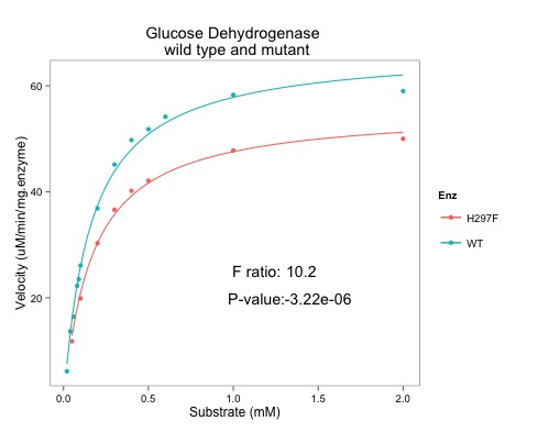
R is good at statistics. I've been learning how to calculate F ratios in R to allow me to compare the lines fitted using glucose hydrogenase wild type and H297F mutant data that we graphed up in the previous blog post.  I want to add the p-value to the plot:

Note the addition of the F ratio and the p-value (very small)

The question from the statistical point of view: is fitting two lines better than fitting just one.

• Our null hypothesis says that one line fits all the data well. 
• The alternative hypothesis says that two lines fits the data well.

The question from an biochemistry experimental point of view: does the mutant glucose dehydrogenase H297F have different properties to wild type. If the mutation has no effect on the enzyme kinetics, then one line should fit all the data well. If not then two lines should fit the line better. This test won't tell us which or how the lines are different, just that they are.

Key steps to answer this question:

1. Fit one line to all the data  (fitTotal)
2. Fit the two lines to the two separate sets of data (fitWT and fitH297F). 
3. Extract the differences (deviance) between the data and the lines (aka sum of squares.)  
1. SS.null <- fitTotal$m$deviance() 
2. SS.alt <- fitWT$m$deviance() + fitH297F$m$deviance()
4. Extract the degrees of freedom for null and alternative hypothesis
1. df.null <- df.residual(fitTotal)
2. df.alt <- df.residual(fitWT) + df.residual(fitH297F)
5. Divide the deviance by the degrees of freedom which is this case is the number of samples less the number of lines we have drawn. This gives us the mean square - the average sum of squares.
1. mean.squares.null <- SS.null/df.null
2. mean.squares.alt <- SS.alt/df.alt
6. The F-ratio is the mean square for the null hypothesis (one line fits all the data) divided by mean squares for the alternative hypothesis.
1. Fratio <- mean.squares.null/mean.squares.alt
7. I calculated the p value if you know the F-ratio and the degrees of freedom using the pf() function.
1. p.val <- pf(Fratio, df.alt, df.null, log.p = TRUE)
8. I added the F-ratio and the p-value to the ggplot using the annotate() function.

If the variation is the basically the same in both cases - no extra value from plotting two lines, then the F-ratio will be approximately one. The higher the F-ratio the better. The p-value corresponding to the F-ratio depends on the degrees of freedom. R can calculate this.

I've learned most of this from Andy Field's book who has, in my opinion, written the easiest to read statistics books. One or two parts even made me laugh and I didn't expect that. Lots of the material is available through his website. You can download his information about ANOVA and F-ratios here.

In case you hadn't guessed from the plots, the F-ratio is significant and the null hypothesis is unlikely to be correct. Two lines describe the data better than one line. Our enzyme kinetic values are different.

Here is the script that does the calculations:

# START OF SCRIPT
# compare two models. 
# need to do an ANOVA...

library(ggplot2)

library(ggthemes)

# data from Dr C Bennett, University of Bath
# Link to published data: http://www.jbc.org/content/285/44/33701.full
# and her thesis: http://opus.bath.ac.uk/27220/

Enz <- c("WT","WT","WT","WT","WT",
         "WT","WT","WT","WT","WT",
         "WT","WT","WT",
         "H297F","H297F","H297F",
         "H297F","H297F","H297F",
         "H297F","H297F")
S <- c(2.00, 1.00, 0.60, 0.50, 0.40, 
         0.30, 0.20, 0.10, 0.09, 0.08, 
         0.06, 0.04, 0.02, 
         0.05, 0.10, 0.20, 
         0.30, 0.40, 0.50, 
         1.00, 2.00)
v <- c(59.01, 58.29, 54.17, 51.82, 49.76, 
         45.15, 36.88, 26.10, 23.50, 22.26, 
         16.45, 13.67, 6.14, 
         11.8, 19.9, 30.3, 
         36.6, 40.2, 42.1, 
         47.8, 50.0)

# assemble the data into a data.frame
enzdata <- as.data.frame(Enz)
enzdata$S <- S
enzdata$v <- v

# fit all the data to one NLS...
MMcurve<-formula(v~Vmax*S/(Km+S))
fitTotal <- nls(MMcurve, enzdata, start=list(Vmax=50,Km=0.2), subset=)
# residual sum-of-square: 328   fitTotal$m$deviance()
# from here: https://stat.ethz.ch/pipermail/r-help/2010-August/249065.html
SS.null <- fitTotal$m$deviance()
# from here: http://stackoverflow.com/questions/21734248/how-to-return-only-the-degrees-of-freedom-from-a-summary-of-a-regression-in-r
df.null <- df.residual(fitTotal)

# split the data and fit WT and H297F data
WT <- subset(enzdata, Enz=="WT")
fitWT <- nls(MMcurve, WT, start=list(Vmax=50,Km=0.2))
# residual sum-of-square: 23.36  

H297F <- subset(enzdata, Enz=="H297F")
fitH297F <- nls(MMcurve, H297F, start=list(Vmax=50,Km=0.2))
# residual sum-of-square: 5.523
# add these together because they are one (alternative) model
SS.alt <- fitWT$m$deviance() + fitH297F$m$deviance()
df.alt <- df.residual(fitWT) + df.residual(fitH297F)

mean.squares.null <- SS.null/df.null
mean.squares.alt <- SS.alt/df.alt

# calculate the F-statistic
# http://stats.stackexchange.com/questions/12398/how-to-interpret-f-and-p-value-in-anova
Fratio <- mean.squares.null/mean.squares.alt

# use pf(q, df1, df2, ncp, lower.tail = TRUE, log.p = FALSE)
p.val <- pf(Fratio, df.alt, df.null, log.p = TRUE)
p.val <- format(p.val, dig=3)
           
# Now, draw the plot AND add the p-value using annotate()

ggplot(data=enzdata,         
       aes(x=S,            
           y=v,            
           colour = Enz)) +  
  geom_point() +            
  xlab("Substrate (mM)") +  
  ylab("Velocity (uM/min/mg.enzyme)") +    
  ggtitle("Glucose Dehydrogenase \n wild type and mutant") +  

  geom_smooth(method = "nls", 
              method.args = list(formula = y ~ Vmax * x / (Km + x), 
                start = list(Vmax = 50, Km = 0.2)),
             se = F, size = 0.5,
             data = subset(enzdata, Enz=="WT"))  +

  geom_smooth(method = "nls", 
                method.args = list(formula = y ~ Vmax * x / (Km + x), 
                                   start = list(Vmax = 50, Km = 0.2)),
                se = F, size = 0.5, 
              data = subset(enzdata, Enz=="H297F")) +
  theme_few() +

            annotate("text", x = 1.15, y = 25, label = "F ratio: ") +
            annotate("text", x = 1.4, y = 25, label = format(Fratio, dig=3)) +
            annotate("text", x = 1.15, y = 20, label = "P-value: ") +
            annotate("text", x = 1.5, y = 20, label = p.val)

# END OF SCRIPT