Showing posts with label visualisations. Show all posts

Thursday, 7 January 2016

Drawing a cytokine receptor with R - TNFR1...

During my research, I have studied the pro-inflammatory cytokine TNF and its receptor, TNFR1. TNF and TNFR1 are involved in inflammatory diseases such as rheumatoid arthritis. As part of developing my skills drawing molecules with R, I have written this script to draw TNFR1.

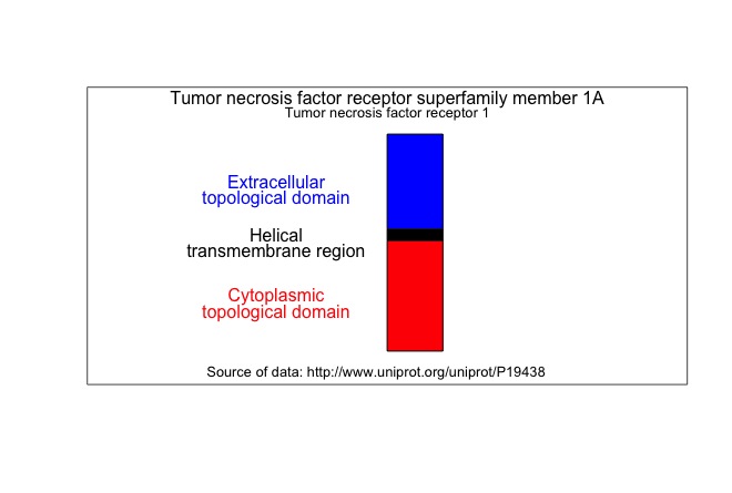
I like to draw receptors vertically with the thought that the cell plasma membrane lies horizontal to the view. The height of the rectangles are proportional to the number of amino acids.

I took the data from the UniProt page for TNFR1. Here is the diagram.


The key functions involved are the 
  • plot() function that creates the space to draw in
  • rect() function that draws a rectangle
  • text() function that adds text at a designated spot. 


Here is the script:
# START
# draw the Tumor Necrosis Factor Receptor 1 with R.
# draw it as a series of rectanges
# vertically rather than horizontal. 

# using the Uniprot webpage for the informaton
# http://www.uniprot.org/uniprot/P19438
# cut and paste from the XML page to create two objects
# first object is a list containing accession number and names


## Step 1: a list containing names 
# list of names...
names <- list(
  accession = c("P19438"),
  name = "TNR1A_HUMAN",
  protein.recommendedName.fullName = "Tumor necrosis factor receptor superfamily member 1A",
  protein.recommendedName.alternativeName = "Tumor necrosis factor receptor 1",
  protein.recommendedName.alternativeName.shortName = "TNF-RI",
  gene.name.primary = "TNFRSF1A",
  gene.name.synonym = "TNFAR",
  organism.name.scientific = "Homo sapiens"
)


## Step 2: getting the details of the molecule
# draw TNFR....
# Topological domain  22  211 Extracellular 189
# Transmembrane 212 234 Helical 22
# Topological domain 235 455 Cytoplasmic 220

# create the data frame with all the information. 
# cut and past from the XML page to make vectors
# features to plot 
types <- c("chain", "topological domain", "transmembrane region", "topological domain") 
description <- c("Tumor necrosis factor receptor superfamily member 1A, membrane form", "Extracellular", "Helical","Cytoplasmic")
begin <- c(22,22, 212, 235)
end <- c(455, 211, 234, 455)
subbegin <- 500 - begin # do these subtractions because we want to draw from top to bottom. 
subend <- 500 - end
col <- c("white", "blue", "black", "red")  # my decision - easy to change. 

# assemble vectors into a data frame
features <- data.frame(types, description, subbegin, subend, col)

# check the structure of the data frame
str(features)
# shows description and col to be factors - this will cause problems later...
# so change them now
features$description <- as.character(features$description)
features$col <- as.character(features$col)  


## step 3: draw the diagram - but vertically
screen.width <- 25 
screen.height <- 550  # this is a bit arbitrary

# we create a plot space to draw in....
plot(c(0, screen.width), 
     c(0, screen.height), 
     type= "n", 
     xlab = "", xaxt = 'n',   # suppress the x label and x axis
     ylab = "", yaxt = 'n')   # suppress the y label and y axis

# make the rectangles in a loop
for (i in 1:length(features$types) ) {
  rect(xleft   = screen.width/2,
       ytop    = features$subbegin[i],
       ybottom = features$subend[i],
       xright  = screen.width/2+2.5,
       col = features$col[i])
}
## Step 4: add text 
# text positioning all for horizontal code
# add text to the top of the illustration with the recommended name
text(screen.width/2, screen.height-2.5, names$protein.recommendedName.fullName, cex=1)
# and the alternative name
text(screen.width/2, screen.height-30, names$protein.recommendedName.alternativeName, cex=0.8)
# and source
text(12, 3, "Source of data: http://www.uniprot.org/uniprot/P19438", cex=0.8)

# add the descriptions of the features and source
# "chain" doesn't really help as a piece of text so going to leave this out. 
pos.text.y <- features$subbegin[2:4] + (features$subend[2:4] - features$subbegin[2:4])/2
pos.text.x <- 7.5
text(pos.text.x, pos.text.y, features$description[2:4], cex=1, col=features$col[2:4])
text(pos.text.x, pos.text.y - 35, features$types[2:4], cex=1, col=features$col[2:4])
## Step 5: add protein domains using shading as detailed on Uniprot
# add more TNF receptor domains:
begin <- c(43, 83, 126, 167, 356)
subbegin <- 500 - begin
end <- c(82, 125, 166, 196, 441)
subend <- 500 - end
description <- c("TNFR-Cys 1", "TNFR-Cys 2", "TNFR-Cys 3", "TNFR-Cys 4", "Death"  )
types <- c("repeat", "repeat", "repeat", "repeat", "domain")
density <- c(10, 10, 10, 10, 5)  # this gives lines in the shading
angle <- c(45, 135, 45, 135, 15) # this gives angles of the lines

features <- data.frame(types, description, subbegin, subend, density, angle)
features$description <- as.character(features$description)

# make the rectangles in a loop
for (i in 1:length(features$types) ) {
  rect(xleft   = screen.width/2,
       ytop    = features$subbegin[i],
       ybottom = features$subend[i],
       xright  = screen.width/2+2.5,
       lwd = 2,
       density = features$density[i],
       angle = features$angle[i]      
       )
}

# add the descriptions of the features
x <- length(features$types)
pos.text.y <- features$subbegin[1:x] + (features$subend[1:x] - features$subbegin[1:x])/2
pos.text.x <- 19.5
text(pos.text.x, pos.text.y, paste(features$description[1:x], features$types[1:x]), cex=1)

# SCRIPT END

Monday, 12 October 2015

What do I tweet about? Not just R...

Here is another script for my talk entitled First steps in making visualisations using R as part of SQLRelay in Cardiff. It's about using R to make a word cloud or wordle.

Here is my word cloud which shows who and what I tweet about:
What I tweet about: too much bread and not enough work?
I downloaded my twitter archive with help from this link. The resulting .csv file is on Github so that it can be downloaded as part of this script.

Below is the script that I used to make the word cloud. It also shows how the word cloud developed - I removed various words that I didn't think were useful. I did this by using the text mining package - tm. I looked at word frequencies and removed the words I didn't like using the tm.map() function.

SCRIPT START:

# if required install.packages(c("wordcloud", "tm", "ggplot2", "RCurl"))

library("wordcloud")
library("tm")
library("ggplot2")
library("RCurl")

x <- getURL("https://raw.githubusercontent.com/brennanpincardiff/RforBiochemists/master/data/tweets.csv")

twts <- read.csv(text = x)

str(twts)
# it's a data.frame

text <- twts$text  # pull out the text... 
str(text)   # check the structure
# factor - no I dont' think that's quite what we want...

text <- as.character(twts$text)
str(text)
# so that worked and looks better 

# check a few of the entries...
text[1]
text[2]
text[10]


# defaults are not great - quite slow and probably too many words to be useful. 
# best to add a max.words modifier....
wordcloud(text, max.words = 35)


wordcloud(text, 
          max.words = 35,
          random.order=FALSE, 
          rot.per=0.35, 
          use.r.layout=FALSE, 
          colors=brewer.pal(8, "Dark2"))


Add some colour and get a nice layout...

# layout is random... 

# some interesting words here
# my name: brennanpcardiff
# some people I communicate with on twitter: amcunningham, drbillyo, drnostromo
# words like amp, just, the, think, well, day, now, nice, great, new

# good to do some processing....

# convert into a Corpus - a structure for organising text...
text.c <- Corpus(VectorSource(text))
text.c.p <- tm_map(text.c, content_transformer(tolower))
# remove stopwords
text.c.p <- tm_map(text.c.p, removeWords, stopwords("english"))
# get a list of Englisth stopwords....
stopwords(kind = "en")
length(stopwords(kind = "en"))

wordcloud(text.c.p, max.words = 35, colors=brewer.pal(8, "Dark2"))


Not quite what I wanted....


# so some words removed but leaving others... including smiley face. 
# remove some Punctuation
text.c.p <- tm_map(text.c.p, removePunctuation)

wordcloud(text.c.p, max.words = 35, colors=brewer.pal(8, "Dark2"))


# better... rstats has appeared - good to see. 
# not sure how useful day, the, can, well, like, http are....
# remove more words
text.c.p <- tm_map(text.c.p, removeWords, c("new", "the", "today", "can","just", "day", "amp", "http", "good", "great", "like", "nice", "well", "brennanpcardiff", "will", "now", "httpt", "get", "one"))

set.seed(501)
wordcloud(text.c.p, 
          max.words = 30,
          random.order=FALSE, 
          rot.per=0.35, 
          use.r.layout=FALSE, 
          colors=brewer.pal(8, "Dark2"))


# for more on word frequencies and a graph....... 

# create Document Term Matrix
dtm <- DocumentTermMatrix(text.c.p)
inspect(dtm)
dim(dtm)

# Plotting Word Frequencies
freq <- sort(colSums(as.matrix(dtm)), decreasing = TRUE)
head(freq, 14)

# make the data frame for ggplot
wf <- data.frame(word = names(freq), freq = freq)
head(wf,20)

wf.freq <- subset(wf, freq > 35) # data frame with abundant words - 23 words

p <-  ggplot(wf.freq, aes(word, freq)) + 
             geom_bar(stat="identity") +
             xlab("Frequent words") +   # label x-axis
             ylab("Frequency") +    # label y-axis
             ggtitle("Word Frequencies in my tweets") +
             theme_bw() +
             theme(axis.text.x = element_text(angle=45, hjust=1)) 

p  # show the object...


# make another wordle with the frequencies... gives the same plot...
set.seed(501)  # gives a reproducible plot...
wordcloud(names(freq), freq, max.words =30,
          random.order=FALSE, 
          rot.per=0.35, 
          use.r.layout=FALSE, 
          colors=brewer.pal(8, "Dark2"))


Helpful resources that I used:


Friday, 2 October 2015

Understanding and visualizing a distance matrix

My PhD student has just received the data from a set of RNA samples analysed using a gene array. We discussed what should be done first to analyse these experiments. A good first step is to look at the distance between the samples and do unsupervised hierarchical clustering of all the samples to see how the biological replicates gather together. This represents an unbiased way to do some quality control for your experiments. Rather than just trying to identify different genes, we use all the data to determine if replicates gather together, if we have any outliers and to find patterns in the data. 

The first step is the generation of a distance matrix. A distance matrix tells us the difference between lists of numbers. If we put together a group of samples, then the distance matrix compares all of the samples. We discussed the purpose of the data matrix and visualising the matrix. I've written the following R script that tries to explain the concept. Mel helped me develop the script to visualise it using a script from this very informative Stack Overload post

Here is the a visualisation of a distance matrix using published data (Webber et al, 2014): 


Visualisation of distance matrix using data from Webber et al, 2014 

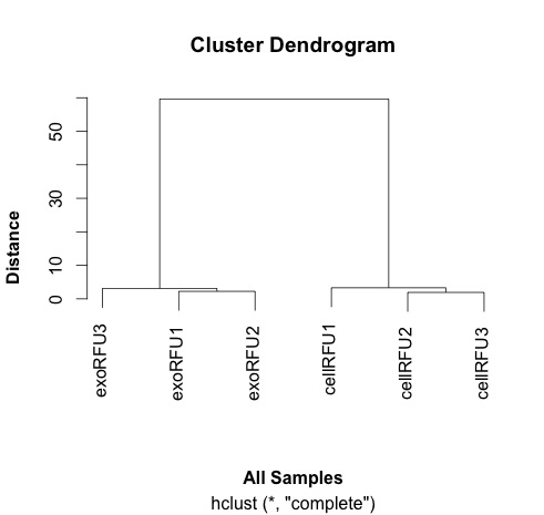
This distance matrix is used to do the hierarchical clustering that is plotted out here and shown here: 


Clustering samples using data from Webber et al, 2014.


# Trying to explain the concept of distance
# simple example 1: one digit different by 2 between two samples
samp1 <- c(0, 1, 2, 3, 4, 5, 6, 7, 8)
samp2 <- c(0, 1, 2, 3, 4, 5, 6, 7, 10)
dist(rbind(samp1, samp2))
# the dist() function compares each of the numbers in order along the two rows of the matrix. 
# answer is in this case is 2, as one number in the list is different by 2 to another. 

# simple example 2: one digit different by 72 between two samples
samp1 <- c(0, 1, 2, 3, 4, 5, 6, 7, 8)
samp2 <- c(0, 1, 2, 3, 4, 5, 6, 7, 80)
dist(rbind(samp1, samp2))
# answer is 72

# a little more complicated: two digits different
samp1 <- c(0, 1, 2, 3, 4, 5, 6, 7, 8)
samp2 <- c(0, 10, 2, 3, 4, 5, 6, 7, 80)
dist(rbind(samp1, samp2))
# now the answer is 72.56
# why? 
# well because of the equation used by the default method. 
# the default for the dist() function is euclidean 
# the equation for this is dist = sqrt(sum(x_i - y_i)^2)
# in this case, this calculates as sqrt(9^2 + 72^2)
# why the sqrt and the sum - in part so that the negatives and the positive differences don't cancel each other out.

# you can use other methods of calculating distance
help(dist)

# another is the "maximum" which just gives us the largest difference between the two arrays
# "Maximum distance between two components of x and y"
samp1 <- c(0, 1, 2, 3, 4, 5, 6, 7, 8)
samp2 <- c(0, 10, 2, 30, 4, 5, 6, 7, 80)
dist(rbind(samp1, samp2), method="maximum")
# in this case 72

# a third is the "manhattan" which sum of the absolute distances between the vectors
# "Absolute distance between the two vectors"
samp1 <- c(0, 1, 2, 3, 4, 5, 6, 7, 8)
samp2 <- c(0, 10, 2, 3, 4, 5, 6, 7, 80)
dist(rbind(samp1, samp2), method="manhattan")
# the answer now is 81

# now just envisage a more complicated situation when there are lots more numbers
# more than two samples and numbers that are higher and lower. 

# let's take a couple of examples from some data we analysed previously:

# http://www.mcponline.org/content/13/4/1050.full
# supplementary data is here: http://www.mcponline.org/content/suppl/2014/02/06/M113.032136.DC1/mcp.M113.032136-5.xlsx
# install if necessary:
# install.packages("readxl")
library(readxl)

# this is the link to the data
link <- "http://www.mcponline.org/content/suppl/2014/02/06/M113.032136.DC1/mcp.M113.032136-6.xlsx"

# the download.file() function downloads and saves the file with the name given
download.file(url=link,destfile="file.xlsx", mode="wb")

# then we can open the file and extract the data using the read_excel() function. 
data<- read_excel("file.xlsx")

View(data)

# the data has 762 observations. 

# we can only calculate distances in a matrix where all the values are the same mode - e.g numbers
# convert data frame (data) into a matrix 
# only want a subset of the data - the data from the samples. 
data.m <- as.matrix(data[2:7])
# transpose the data because a distance matrix works in rows
data.m.t <- t(data.m)

# calculate the distances and put the calculations into an object called distances
distances <- dist(data.m.t)

# convert this distances object into a matrix. 
distances.m <- data.matrix(distances)

# you can look at this object.
View(distances.m)

# we can extract the size of the object and the titles
dim <- ncol(distances.m)
names <- row.names(distances.m)

# now to create the visualisation of the difference matrix. 
# first the coloured boxes
image(1:dim, 1:dim, distances.m, axes = FALSE, xlab = "", ylab = "")

# now label the axis
axis(3, 1:dim, names, cex.axis = 0.8, las=3)
axis(2, dim:1, names, cex.axis = 0.8, las=1)

# add the values of the differences
text(expand.grid(1:6, 6:1), sprintf("%0.1f", distances.m), cex=1)

# this example lacks subltety
# the exo samples are very close together and the cell samples are quite far apart.
# it explains why the cluster analysis is so dramatic. 

# export this image as a tiff file with width of 1000 seems to work well. 
# some of the other formats don't work as well. 

# to make the cluster dendrogram object using the hclust() function
hc <- hclust(distances) 
# plot the cluster diagram
# some interesting groups in the data
plot(hc, 
     xlab =expression(bold("All Samples")), 
     ylab = expression(bold("Distance")))
# replicates cluster together well. 


The visualisation was inspired by this:


If you have feedback on this script, please leave a comment. 


Friday, 11 September 2015

Downloading and manipulating published proteomic data...

Update: 1 July 2025 - so a lot has happened in 10 years. This includes people moving jobs, promotions and the reorganisation of data on published website. 

Aled was promoted to Professor at Cardiff University 

----

There are many ways to get data into R. I want to illustrate a method of downloading published data within R, opening the data (an Excel file) and then doing visualisations and manipulations. 

I have chosen a paper from Molecular and Cellular Proteomics which uses aptamers to detect multiple proteins in exosomes and cells. 

The data was generated by colleagues that were working in the School of Medicine at Cardiff University including the first author - Dr Jason Webber, a Prostate Cancer UK funded Research Fellow and senior author, Professor Aled Clayton, a Senior Lecturer in Cancer & Genetics at Velindre Hospital. Dr Tim Stone was key to the data analysis. The protein detection method is from a company called SomaLogic

The first step was downloading the file from the Molecular and Cellular Proteomics website. I used the download.file() function. This saves the file into your current directory. This was opened using the readxl package (by Hadley Wickham) using the read_excel() function. 

I drew some graphs as I explored and manipulated the data. These are interspersed with the script below.  The visualisations included boxplots and a cluster diagram. 

I wanted to draw a volcano plot which expresses the fold change against the significant of the change (p-value). I couldn't do that with the data supplied so I had to reverse the transformation and calculate the fold change again. 

Here is the volcano plot:
Comparison of changes in exosomes compared cells. Proteins over-expressed in exosomes are on the right. Proteins over-expressed in cells are on the left. 

The plot indicates that there are more proteins over-expressed in cells (on the left) compared to exosomes (on the right). 

Update: 1 July 2025 - orignally, I was able to download the data directly from the Molecular and Cellular Proteomics website. However, at some point, they reorganised their site and put all the data into a zip file. This means that downloading it requires multiple steps outside of R. To make this analysis more stand alone, I have down loaded the data from this zip file and uploaded the spreadsheet onto my Github site. This means that the script will download and analyse the data. 

Here is the script with some other plots along the way:

START
# pull down a file from the internet, do some analysis and draw a graph...
# choose Jason Webber's MCP Paper...
# the data can be downloaded using this link with give zip file. 
# It isn't necessary to do that for this script. 
# install if necessary:
# install.packages(c("ggplot2", "readxl")) 
library(ggplot2)
library(readxl)


# this is the link to the data
link <- "https://github.com/brennanpincardiff/RforBiochemists/raw/master/R_for_Biochemists_101/data/mcp.M113.032136-6.xlsx"

# the download.file() function downloads and saves the file with the name given
download.file(url=link,destfile="file.xlsx", mode="wb")

# then we can open the file and extract the data using the read_excel() function. 
data<- read_excel("file.xlsx")

View(data)

# plot the data - always an important first step!
boxplot(data[2:7], 
        las =2, # las = 2 turns the text around to show sample names
        ylab = expression(bold("expression")),
        main="Boxplot of expression data")  


Two types of sample - exosomes (n=3) and cells (n=3).

# do a cluster analysis to quality control the different groups
# convert to matrix first
data.m <- as.matrix(data[2:7])
dim(data.m)   # gives the dimensions of the matrix
# ans: 762   6

# calculate the distances using the dist() function. 
# various methods are possible - default is Euclidean. 
distances <- dist(data.m)
summary(distances) # have a look at the object

# make the cluster dendrogram object using the hclust() function
hc <- hclust(distances) 
# plot the cluster diagram
# some interesting groups in the data
plot(hc, 
     xlab =expression(bold("All Samples")), 
     ylab = expression(bold("Distance")))


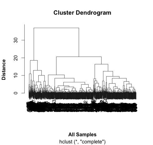
# ah, not what I intended. 
# it clustered the proteins NOT the samples. 

# transpose the data and try again...
data.m.t <- t(data.m)
dim(data.m.t)
# ans = 6  762 - so that has worked. 
# repeat cluter analysis

# calculate the distances using the dist() function. 
# various methods are possible - default is Euclidean. 
distances <- dist(data.m.t)
summary(distances)

# make the cluster dendrogram object using the hclust() function
hc <- hclust(distances) 
# plot the cluster diagram
# some interesting groups in the data
plot(hc, 
     xlab =expression(bold("All Samples")), 
     ylab = expression(bold("Distance")))
# replicates cluster together well. 


# the adjusted P value are in a column entiteld: BH - P.value
# this is a little awkward so rename this and Fold Change column:
colnames(data)[9] <- "P.Value"
colnames(data)[10] <- "Fold.Change"
plot(data$P.Value ~ data$Fold.Change)


# this works but we would like to turn it into a volcano plot 
# with log2 at the bottom and -p-value. 
# we can't log fold changes as half of them are negative numbers 
# we need to re-calculate the raw data
# reverse the log2 transformation. 
# mean the values & calculate fold change in decimal format (no +/-)
data$exo1 <- 2^data$exoRFU1
data$exo2 <- 2^data$exoRFU2
data$exo3 <- 2^data$exoRFU3
data$cell1 <- 2^data$cellRFU1
data$cell2 <- 2^data$cellRFU2
data$cell3 <- 2^data$cellRFU3

# calculate means of the replicates
data$exoMean <- rowMeans(data[,13:15])
data$cellMean <- rowMeans(data[,16:18])

# always good to visualise the data:
plot(log2(data$exoMean)~log2(data$cellMean))


# calculate fold change exo/cell
data$FoldChange <- data$exoMean/data$cellMean
plot(log2(data$FoldChange)) # transform for plotting


# make column in data.frame with transformed data
data$Log2.Fold.Change <- log2(data$FoldChange)

## Identify the genes that have a p-value < 0.05
data$threshold = as.factor(data$P.Value < 0.05)


## Construct the volcano plot object using ggplot
g <- ggplot(data=data, 
            aes(x=Log2.Fold.Change, y =-log10(P.Value), 
                colour=threshold)) +
  geom_point(alpha=0.4, size=1.75) +
  xlim(c(-6, 6)) +
  xlab("log2 fold change") + ylab("-log10 p-value") +
  theme_bw() +
  theme(legend.position="none") + 
  ggtitle("Volcano Plot comparing protein expression in exosomes vs cells ")  # add a title
  
g # show the plot 

END of script

So I think that the threshold of p<0.05 is too low for this volcano plot. It's relatively easy to change and would make a good exercise. Perhaps a threshold of p<0.00001 would be better. 


Useful resources (updated 1 July 2025)

Tuesday, 23 June 2015

My first cluster diagram

For our CLL proteomic manuscript we were asked to do some more statistical analysis (Proteomics-Based Strategies To Identify Proteins Relevant to Chronic Lymphocytic Leukemia Alsagaby et al, J. Proteome Res., 2014, 13 (11), pp 5051–5062).

The reviewer particularly recommended hierarchial clusteringFortunately, I had been learning how to use R, so I was able to learn how to do this relatively easy. This was why I had chosen to learn R.  

"The idea of a cluster diagrams is to build a hierarchy of clusters, showing relations between the individual members and merging clusters of data based on similarity." I learned this from a website that seems to have disappeared now.

Cluster diagrams can be used to investigate the quality of your data and identify outliers in sets of data. They can also show patterns and identify groups of samples.

A key concept is a "distance metric" which is a measure of similarity. There are different measures of correlation. Two common ones are the Euclidean and the Pearson correlations. Euclidean distance looks at just the numbers while the Pearson correlation looks more at trends. This can give very different patterns. Other measures of distance include: maximum, Manhattan, Canberra, binary and Minkowski.

The first step is calculate a distance matrix using the dist() function.

Then you can use this matrix to do the clustering using the hclust() function.

Finally, you plots this: plot(hc).

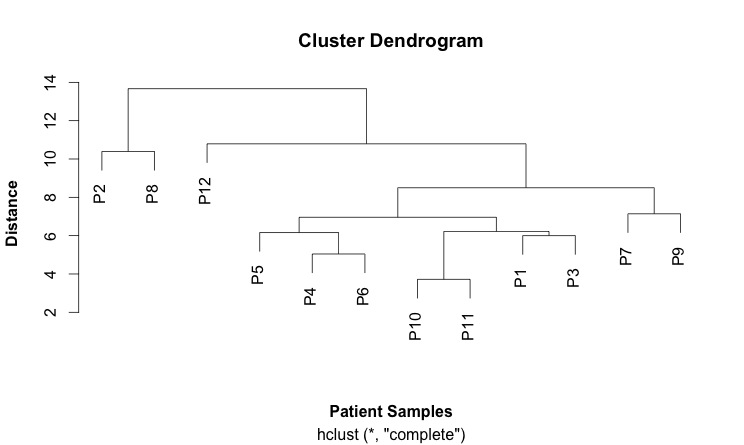
This is my first cluster diagram:


Here is the script that generates it:

SCRIPT
# import the data
link <- ("https://raw.githubusercontent.com/brennanpincardiff/RforBiochemists/master/data/iTRAQPatientforCluster.csv")

data2 <- read.csv(link, header=TRUE)

attach(data2)  # attaching a data.frame means we can use the headings directly. 
head(data2)  # look at the top of the file. 

# first step is to calculate the distances using the dist() function. 
# various methods are possible - default is Euclidean. 
distances2 <- dist(rbind(P1, P2, P3, P4, P5, P6, P7, P8, P9, P10, P11, P12))
distances2
summary(distances2)

# make the cluster dendrogram object using the hclust() function
hc <- hclust(distances2)  

# plot the cluster dendrogram object using base graphics
plot(hc, xlab =expression(bold("Patient Samples")), ylab = expression(bold("Distance")))

detach(data2) # good practice to detach data after we're finished.