Colouring my kinome phylogenetic tree...

I have been playing with the kinome phylogenetic tree that I made last week inspired by the paper in Science from Manning et al in 2002. The first thing I want to do is to add color to the lines. This has proved a bit more difficult than I had anticipated and was a steep learning curve. It reminds me that data visualisation is a real combination of art, science, coding, time and effort.

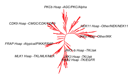
Here is a coloured kinome tree that I am kind of happy with for the moment. I think there is some improving still to do but it's nicer than the one coloured version I made before.

The code below uses a very manual approach to manipulating trees. There are various reasons for that and these include the fact that I want to make an unrooted tree. There are ways to manipulate trees using other packages including phytools and ggtree. However, I'm not able to get them to work well with unrooted trees. There is still more to learn....

Here is the code that I used to draw this and some of the trees that I made along the way:

START
library(ape)
library(RCurl)

# a tree was made using code in a previous blog post. 
# see here: http://rforbiochemists.blogspot.co.uk/2017/01/visualizing-kinome-in-r-simple-tree.html
# it's here on github
link <- "https://raw.githubusercontent.com/brennanpincardiff/RforBiochemists/master/phyloTrees/kinaseTree_20161221"

# this will download it into R. 
# using read.tree() from ape package
tree <- read.tree(file = link)

# this tree looks quite nice in my opinion and is the starting point of this blog 
plot(tree, "u", 
     use.edge.length = FALSE,
     show.tip.label = FALSE,
     edge.color = "red")
# but lacking colours for the groups and any labels...

# it seems more traditional to draw trees from left to right. 
plot(tree, 
     use.edge.length = FALSE,
     show.tip.label = FALSE,
     edge.color = "red")

# with some names... this is slow to draw due to the names 
plot(tree, 
     use.edge.length = FALSE,
     edge.color = "red",
     cex = 0.25)

# and you can't read the names because there are >500

# to customise this tree in a way we want we need to understand a little more about trees
# we can find out more about an object by writing the name
tree
# "Phylogenetic tree with 516 tips and 514 internal nodes"

# by using the class() function
class(tree)
# "phylo"

# or by using the str() structure function
str(tree) 
# "List of 4"
# this list includes $edge, $Nnode, $ tip.label and $edge.length
# the tree$tip.label includes family designation
tree$tip.label  # 516 of these

# from the Science paper, we have seven kinase families:
# kinase categories... TK, TKL, STE, CK1, AGC, CAMK, CMGC
# with the following colours
# "red", "green", "paleblue", "orange", "yellow", "purple", "pink", "green" 


# by using the grep()function on the tree$tip.label part of the object
# we can find the tip labels that include "TK/" - i.e. tyrosine kinases
grep("TK/", tree$tip.label)  # gives a list of numbers with "TK/" in tip label
length(grep("TK/", tree$tip.label))
# thus there are 94 tip labels with that are designated TK (not TKL tyrosine kinase like)

# make a vector for each tip.label called tipcol with black on all of these...
tipcol <- rep('black', length(tree$tip.label))

# make a vector with our list of kinase categories
kinaseCats <- c("TK/", "TKL", "STE", "CK1", "AGC", "CAMK", "CMGC", "RGC")

# make a vector of color we want:
colorsList <-c("red", "darkolivegreen3", "blue", "orange", "yellow", "purple", "pink", "green")

# replace colours where grep gives "TK" as red, etc in a loop
for(i in 1:length(kinaseCats)){
  tipcol[grep(kinaseCats[i], tree$tip.label)] <- colorsList[i]
}

# plot with edge length false to see nodes better
plot(tree, 
     use.edge.length = FALSE,
     tip.color=tipcol, 
     cex = 0.25)
# slow to draw due to text - a bit annoying!

Kinome tree with different coloured labels for different kinds of kinases. Tyrosine kinases are in red. 

# trees are made up of nodes and edges. 
# its possible to label nodes using nodelabels() function from ape package
nodelabels(cex=0.4)
# labels internal nodes. 

Internal nodes of the tree are labelled with the number

# the only way seems to identify the relevant nodes manually
# i.e. the nodes that include the kinase groups that we have coloured
# from the bottom
# for 1st "green" looks like node 574
# for "red" looks like node 607
# for 2nd "green" somethink like 701 but very difficult to see
# for "purple" most of 749 and also north of 726 but I can't read the number
# "blue" node 723
# "yellow" node 885, I think
# "pink" node 955, I think
#  not perfect but getting there....

# adding edge colors
# from 111 to 177 should be green
# from 178 to 364 should be red. 
# from 459 to 577 should be purple
# from 578 to 608 should be purple too
# from 641 to 733 should be blue
# from 735 to 850 approx should be yellow
# from 876 to 980 should be pink
# http://stackoverflow.com/questions/34089242/phylogenetic-tree-tip-color
# make a vector for each edge called edgecol with black on all of these...
edgecol <- rep('black', nrow(tree$edge))
edgecol[178:364] <- "red" # "TK/"
edgecol[111:177] <- "green" # "TKL" OR "RGC"
edgecol[641:733] <- "blue" # "STE"
edgecol[1003:1029] <- "orange" # "CK1"
edgecol[735:850] <- "yellow" # "AGC"
edgecol[459:577] <- "purple" # "CAMK"
edgecol[578:608] <- "purple" # "CAMK"
edgecol[876:980] <- "pink" # "CMGC"


plot(tree,
     use.edge.length = FALSE,
     tip.color=tipcol, 
     edge.color = edgecol,
     cex = 0.25)

Kinome Tree with text and branches coloured. 

plot(tree, "u",
     use.edge.length = FALSE,
     tip.color=tipcol, 
     edge.color = edgecol,
     cex = 0.25)

# plot.phylo() function from ape package allows rotation of tree. 

plot.phylo(tree, "u", 
           use.edge.length = FALSE,
           edge.color = edgecol,
           rotate.tree = -95,
           show.tip.label = FALSE)

# want to add some names at the ends of the branches
# try to find out some tip numbers using
tiplabels(cex=0.3)

# add labels to node 246, 105, 191 and 340
tree$tip.label[246] # "CaMK1d_Hsap_-CAMK/CAMK1"
tree$tip.label[105] # "EphA3_Hsap_-TK/Eph"
tree$tip.label[191] # "TGFbR1_Hsap_-TKL/STKR/Type1"
tree$tip.label[340] # "TNIK_Hsap_-STE/STE20/MSN"

# add these to a list
kinaseLabels <- c("IKKa","ErbB2", "MLK1", "PKCb", 
                  "CDK9", "CaMK1d_Hsap_-CAMK/CAMK1",
                  "EphA3_Hsap_-TK/Eph", "TGFbR1_Hsap_-TKL/STKR/Type1",
                  "TNIK_Hsap_-STE/STE20/MSN")

# extract tip.labels
tipLabels <- tree$tip.label

# find these in the alignment - they will be tip labels
labelNo <- NULL
for(i in 1:length(kinaseLabels)){
  labelNo <- c(labelNo, grep(kinaseLabels[i], tree$tip.label))
}
# generates a vector of 9 numbers. Some labels in two names. 

# make a vector of blank tiplabels
tipLabels_2 <-  rep('', length(tree$tip.label))

# add the labels we want to the vector...
for(i in 1:length(labelNo)){
  tipLabels_2[labelNo[i]] <- tipLabels[labelNo[i]]
}

# make a new tree
tree_fewLabels <- tree

# replace the tip labels with the shorter list.
tree_fewLabels$tip.label <- tipLabels_2

# remove "Hsap" 
tipLabels_2 <- gsub("Hsap", "", tipLabels_2)
tree_fewLabels$tip.label <- tipLabels_2

# plot.phylo() function from ape package allows rotation of tree. 
plot.phylo(tree_fewLabels, "u", 
           use.edge.length = FALSE,
           edge.color = edgecol,
           rotate.tree = -95,
           show.tip.label = TRUE,
           cex = 0.4)

# add a title and source
plot.phylo(tree_fewLabels, "u",
     main="Phylogenetic tree of human kinase domains",
     sub="source: www.kinase.com & Manning et al Science (2002) 398:1912-1934",
     rotate.tree = -95,
     use.edge.length = FALSE,
     edge.color = edgecol,
     show.tip.label = TRUE, font = 2,
     cex = 0.5)

# this looks quite good and is enough for today. 

Visualizing the kinome in R - a 'simple' tree...

A paper by Manning et al in Science in 2002 showed an phylogenetic tree of the kinases in the human genome. With the help of a beautiful poster and web resources by Cell Signaling Technologies, this visualisation has become a classic among researchers working on protein kinases.

It has been used in many ways and the paper itself has be very extensively cited.
Examples include:

• Plant and animal pathogen recognition receptors signal through non-RD kinases.
• Global target profile of the kinase inhibitor bosutinib in primary chronic myeloidleukemia cells
• Kinase binding selectivity for representative inhibitors shown on the human kinome dendrogram

This blog post uses the sequences available on the protein kinase website (kinase.com) to create a tree using R. My hope is that this will be the first of few posts that will develop into being able to reproduce the visualisation from the Science and to render a similar image to that created by Cell Signaling Technology. This is really a key objective for me as I want to use this visualisation for my teaching.

If you are interested, please test the code and make comments. This is an ongoing project and I welcome feedback.

So here is the first version of the kinome phylogenetic tree:

I have made a more simple phylogenetic tree of the human proteins with the rel homology domain here which talks about the complexity of making trees.



Here is the script that makes this:
SCRIPT START

library(seqinr)  
library(msa)
library(ape)

# first version of generating a the kinome visualisation in R
# data is here: http://kinase.com/kinbase/FastaFiles/Human_kinase_domain.fasta
# in fasta format...
# need to extract the data into R... 
# need Biostrings package - downloaded as part of seqinr package

file <- c("http://kinase.com/kinbase/FastaFiles/Human_kinase_domain.fasta")

# step 1 is read in the FASTA files. 
kinases <- readAAStringSet(file, format = "fasta")
# that seems to work. 
kinases
# 516 sequences. 
# good.  

# step 2 do the multiple sequence alignment
kinaseAlign <- msa(kinases)  
# takes a bit of time!  - about 3.5 min on my computer...
# currently using default substitution matrix and CLUSTALW 
# creates an object with Formal class 'MsaAAMultipleAlignment' [package "msa"] with 6 slots

# step 3: convert Msa Alignment object into alignment for seqinr 
kinaseAlign2 <- msaConvert(kinaseAlign, type="seqinr::alignment")
class(kinaseAlign2) # it's an alignment
# worked 
# List of 4

# step 4: compute distance matrix - dist.alignment() function from the seqinr package:
d <- dist.alignment(kinaseAlign2, "identity")
# Class 'dist'

kinaseTree <- nj(d)  # from ape package, I think...
class(kinaseTree)
# class "phylo"
# List of 4

# good idea to save the tree locally... remove comment symbol
# write.tree(kinaseTree, file = "kinaseTree")
# to read back in:
# kinaseTree <- read.tree(file = "kinaseTree")

plot(kinaseTree, 
     main="Phylogenetic Tree of kinases")
# too difficult to read so remove the tip.labels which are the kinase names.

plot(kinaseTree, 
     main= "Phylogenetic Tree of kinases", 
     show.tip.label = FALSE)

plot(kinaseTree, 
     type = "unrooted", 
     main= "Phylogenetic Tree of kinases", 
     show.tip.label = FALSE)

# looks quite stylish a a little similar to visualisation in the Science paper
plot(kinaseTree, "u", 
     use.edge.length = FALSE,
     show.tip.label = FALSE)

# need to add colour
# argument is edge.color
plot(kinaseTree, "u", 
     use.edge.length = FALSE,
     show.tip.label = FALSE,
     edge.color = "red")

# want to add selected labels to give some orientation 
# extract tip.labels
tipLabels <- kinaseTree$tip.label

# add some labels we like to orient ourselves:
kinaseLabels <- c("IKKa","JAK3","ErbB2", 
                  "NEK11", "MLK1", "PKCb", 
                  "CDK9", "FRAP")

# find these in the alignment - they will be tip labels
labelNo <- NULL
for(i in 1:length(kinaseLabels)){
  labelNo <- c(labelNo, grep(kinaseLabels[i], kinaseTree$tip.label))
}
# generates a vector of 9 numbers. Some labels in two names. 

# make a vector of blank tiplabels
tipLabels_2 <-  rep('', length(kinaseTree$tip.label))

# add the labels we want to the vector...
for(i in 1:length(labelNo)){
  tipLabels_2[labelNo[i]] <- tipLabels[labelNo[i]]
}

# make a new tree
kinaseTree_fewLabels <- kinaseTree

# replace the tip labels with the shorter list.
kinaseTree_fewLabels$tip.label <- tipLabels_2

# make the plot with these
plot(kinaseTree_fewLabels, "u", 
     use.edge.length = FALSE,
     show.tip.label = TRUE,
     edge.color = "red",
     cex = 0.7)

# remove "Hsap" using gsub() function 
tipLabels_2 <- gsub("Hsap", "", tipLabels_2)
kinaseTree_fewLabels$tip.label <- tipLabels_2
plot(kinaseTree_fewLabels, "u", 
     use.edge.length = FALSE,
     show.tip.label = TRUE,
     edge.color = "red",
     cex = 0.7)

# add a title and source and you have the image at the top...
plot(kinaseTree_fewLabels, "u",
     main="Phylogenetic tree of human kinase domains",
     sub="source: www.kinase.com & Manning et al Science (2002) 398:1912-1934",
     use.edge.length = FALSE,
     show.tip.label = TRUE,
     edge.color = "red",
     cex = 0.7)

# this looks quite good and is enough for today. 

Drawing a simple phylogenetic tree of the human rel homology domain family

Exploring protein structure and protein sequences by making phylogenetic trees is not trivial but can be interesting and informative. It can be a productive way of deepening our understanding of the proteins and the relationships between them.

As a starting point for this blog post, I have chosen to draw a phylogenetic tree of the ten human proteins containing a rel homology DNA binding domain. This family includes the NF-kappaB family of transcription factors and the NFAT family of transcription factors. Both of these families change gene expression in the response to extracellular stimuli. The cytokine, tumor necrosis factor alpha (TNF), activates the NF-kappaB family of transcription factors. Stimulation of cells through antigen receptors, for example the T-cell receptor, activates the NFAT family of transcription factors.

Here is the phylogenetic tree that I have drawn:

It has been generated using the full length protein sequences which is an important point. The proteins are as follows (5 NF-kappaB family members & 5 NFAT family members):

• NF-kappaB subunit p105/p50 - P19838 (NFKB1_HUMAN)
• NF-kappaB subunit p100/p52 - Q00653 (NFKB2_HUMAN)
• NF-kappaB subunit Rel B - Q01201 (RELB_HUMAN)
• NF-kappaB subunit p65/Rel A - Q04206 (TF65_HUMAN)
• NF-kappaB subunit c-Rel - Q04864 (REL_HUMAN)
• NF-ATc1 - O95644 (NFAC1_HUMAN)
• NF-ATc2 - Q13469 (NFAC2_HUMAN)
• NF-ATc3 - Q12968 (NFAC3_HUMAN)
• NF-ATc4 - Q14934 (NFAC4_HUMAN)
• NFAT5 - O94916 (NFAT5_HUMAN)

As a biochemist, protein function is my area of interest and not phylogenetic analysis. The generation of phylogenetic trees has been the subject of many years of research and many books have been written about the topic. There is a book about how to do phylogenetic analysis in R. As such this blog post is just a very brief introduction to how to do this. The idea of this piece is to be inspiring (hopefully) not exhaustive.

The steps are as follows:

1. Get the sequences into R. I’m using the package seqinr to extract protein sequences. The ways in which phylogenetics analysis is done is quite different depending on whether you are using DNA or protein sequences so it’s important to be aware of this.
2. Perform a multiple sequence alignment. I’ve used the msa package. This process compares one sequence to another to another. There are different mathematical methods of doing this and different values that can be used within the different mathematical methods. The msa() function, by default, runs ClustalW with default parameters, one of the standard methods in biology. ClustalW has been around for many years. I first used it about 20 years ago when I did a short online course in bioinformatics. It can be used in my different tools including some web based interactive tools. The msa package also allows the use of the methods ClustalOmega or MUSCLE.
3. Turn your alignment into a tree. This uses the alignment to calculate ‘distances’ between the proteins. The seqinr package has a method and the ape package is used too for neighbor-joining tree estimation. This is not a trivial matter as some changes between amino acids are more likely than others depending on the codon usage. Also some changes may lead a more dramatic change in function than others. Again, there are various algorithms.
4. Draw your tree. This uses the ape package. For a small tree this is relatively simple but for larger trees there can be an artistic element to this. There are many options and a few are illustrated below.

Here is the script that I used to generate the tree above. There are other trees generated along the way...

SCRIPT START
### generating a phylogenetic tree of human Rel homology containing proteins

## packages required - may need downloading
# source("http://www.bioconductor.org/biocLite.R")
# biocLite("msa")

library(seqinr)  
library(msa)
library(ape)

### Get the sequences into R. 
# these are the accession numbers of the 10 proteins. 
# for these 10 proteins I found them manually by searching the Uniprot database
accNo <- c("AC=P19838 OR AC=Q00653 OR AC=Q01201 OR AC=Q04206 OR AC=Q04864 OR AC=O95644 OR AC=Q13469 OR AC=Q12968 OR AC=Q14934 OR AC=O94916")

# using the seqinr package
# From Chapter 4 of the seqinr handbook. 
# http://seqinr.r-forge.r-project.org/seqinr_3_1-5.pdf
### step 4.1 Choose a bank
choosebank()  # show's available data bases
mybank <- choosebank(bank = "swissprot")
str(mybank)
# UniProt Knowledgebase Release 2016_08 of 07-Sep-2016 Last Updated: Oct  4, 2016

### step 4.2 Make the query
mybank <- choosebank(bank = "swissprot")
rel_seq <- query("relSeq", accNo)
# N.B. protein info NOT returned in the same order as requested

# returns list object with six parts 
rel_seq$nelem # with 10 elements - thus 10 proteins
rel_seq$req  # gives the five necessary names

###  4.3 Extract sequences of interest
rel_seqs <- getSequence(rel_seq)
# check the names of the sequences
getName(rel_seq)

# it is necessary to put the sequences in fasta format
# for the multiple sequence alignment.
# useful to store them locally so that's what this does
write.fasta(sequences = rel_seqs, 
            names = getName(rel_seq),
            nbchar = 80, file.out = "relseqs")

### with sequences in a file we can open the file in the package msa

### read in Rel sequences from the file
mySeqs <- readAAStringSet("relseqs")   # from package Biostrings
length(mySeqs)
# 10 sequences... which is correct

### Perform a multiple sequence alignment
myAln <- msa(mySeqs)  
# this uses all the default settings and the CLUSTALW algorithm 
myAln
print(myAln, show="complete")

### Turn your alignment into a tree
# convert the alignment for the seqinr package
myAln2 <- msaConvert(myAln, type="seqinr::alignment")
# this object is a list object with 4 elements

# generate a distance matrix using seqinr package
d <- dist.alignment(myAln2, "identity")
# From the manual for the seqinr package
# This function computes a matrix of pairwise distances from aligned sequences
# using similarity (Fitch matrix, for protein sequences only) 

# have a look at the output
as.matrix(d)

# generate the tree with the ape package
# the nj() function allows neighbor-joining tree estimation
myTree <- nj(d)

# plot the tree
plot(myTree, main="Phylogenetic Tree of Human Rel Homology Domain Sequences")

# since all the species are human, 
# it might be easier to read without the "_HUMAN"
# with the sub() function
myAln2$nam <- sub("_HUMAN", "", myAln2$nam)

# pile up the functions to make a new tree
tr <- nj(dist.alignment(myAln2, "identity"))

# plot the new tree
plot(tr, main="Phylogenetic Tree of Human Rel Homology Domain Sequences")

# selected other ways to draw trees
# from http://ape-package.ird.fr/ape_screenshots.html

plot(tr, "c")

plot(tr, "u")   # unrooted tree 

plot(tr, "c", FALSE)  # ignores edge length

plot(tr, "u", FALSE)

plot(tr, "f", FALSE, cex = 0.5)

plot(tr,               # object with the tree information
     "u",              # unrooted - draws from the centre
     font = 2,         # makes font bold  
     edge.width = 2,   # makes thicker lines
     cex = 1.25,       # increase font size a little
     main = "Phylogenetic Tree of Human Rel Homology Domain Sequences")       

# looks quite stylish but I'm not sure about ignoring edge length
plot(tr, "u", 
     use.edge.length = FALSE, 
     font = 2, 
     edge.width = 2,
     main = "Phylogenetic Tree of Human Rel Homology Domain Sequences")

SCRIPT END


Resources and citations:

• seqinr package: http://seqinr.r-forge.r-project.org/
• msa package: https://bioconductor.org/packages/devel/bioc/vignettes/msa/inst/doc/msa.pdf
• msa package: U. Bodenhofer, E. Bonatesta, C. Horejsˇ-Kainrath, and S. Hochreiter (2015). msa: an R package for multiple sequence alignment. Bioinformatics 31(24):3997–3999. DOI: bioinformatics/btv494.
• ape package: http://ape-package.ird.fr/
• ape package: Paradis, E., Claude, J. and Strimmer, K. (2004) APE: analyses of phylogenetics and evolution in R language. Bioinformatics, 20, 289–290
• ape package: Popescu, A.-A., Huber, K. T. and Paradis, E. (2012) ape 3.0: new tools for distance based phylogenetics and evolutionary analysis in R. Bioinformatics, 28, 1536-1537.