Extracting fluorescence of objects from an Image with R...

In the last blog post, I showed how to identify regions in an image of cells.
This is the image:

It shows about 40 or so cells stained for a protein of interest.

Using the R package, EBImage, it's possible to identify these bright images, count the numbers and then extract and calculate the fluorescence signal in each region.

Here is a graph of the fluorescence signal for each of the 41 regions:

The script that does this is here:

SCRIPT START
# showing how to extract features from an image with EBImage

library(EBImage)
library(ggplot2)

# load up image
# the readImage( ) function will work on URLs to import image into R
c2 <- readImage("https://raw.githubusercontent.com/brennanpincardiff/RforBiochemists/master/data/images/Dros_c2.tif") 
# creates an object called c2

# show a brighter version of the image in the R graphics window
display(c2*4, method = "raster")  #"raster" method means within R

# create the "mask" of this image by blur, threshold and counting
c2.b <- gblur(c2*2, sigma = 5)  #blur
c2.t <- c2.b > otsu(c2.b) # apply otsu threshold 
c2.t.cnt <- bwlabel(c2.t) # count the 'regions'

# show this as a coloured blobs 
display(colorLabels(c2.t.cnt), method = "raster") 
display(colorLabels(c2.t.cnt))  # in a browser

# next step is to extract some of the features about these objects. 
# first extract the basic features (as defined by EBImage). 
# first of these is mean intensity (fluorescence per pixel for the object. )
# this function creates a matrix with each object in a row
# these are calculated using the thresholded image and the original image
ftb <- computeFeatures.basic(c2.t.cnt, c2)

# to get a vector of the mean intensities
m.intent <- ftb[,1]
m.intent # show in Console
# there is one value for each shape...

# next category is shapes
# these a calculated from the thresholded image
fts <- computeFeatures.shape(c2.t.cnt)
area <- fts[,1]  # select first column from object called fts
perimeter <- fts[,2] # select second colum from object called fts

# put the data into a dataframe (a different kind of R object)
df <- as.data.frame(m.intent)
df$area <- area
df$signal <- df$m.intent * df$area
df$regions <- seq(1:nrow(df))

# lots of ways to plot but one of the best is ggplot2
# plot the area of each region on the mask
ggplot(df, 
       aes(x = regions, y=area)) +
  geom_bar(stat="identity")

# plot the signal of each region on the mask
ggplot(df, 
       aes(x = regions, y=signal)) +
  geom_bar(stat="identity")

# plot mean intensity
ggplot(df, 
       aes(x = regions, y = m.intent)) +
  geom_bar(stat="identity")

# dot plot of area v signal
ggplot(df, 
       aes(x=area, y=signal)) +
  geom_point()

# plot the signal of each region on the mask 
# in a slightly nicer way
ggplot(df, 
       aes(x = regions, y=signal)) +
  geom_bar(stat="identity") +
  ggtitle("Fluorescence within each region of the image") + 
  xlab("Regions from top right to bottom left of the image") +
  ylab("Total fluorescence in the region") +
  theme_bw()

# for some help on ggplot2, this R-Cookbook site is good. 
# http://www.cookbook-r.com/Graphs/Bar_and_line_graphs_(ggplot2)/
SCRIPT END

There is lots of extra information about the features that can be extracted here:

• EBImage Reference Manual

Counting and identifying stained cells step by step

On Friday, Dr Joaquín de Navascués and I held the first of two Image Analysis Workshops at Cardiff University. We had a good audience with PhD students and researchers. Joaquin led the first session which explored the fundamentals of images and using Image J or Fiji to open and explore those images.

Key points included:

• good images start at the microscope - try not to over saturate your images during collection.
• protect your original files as it can be easy to alter them permanently and lose data.
• digital pictures are arrays of numbers. 
• these numbers can be visualised and transformed in lots of different ways. 

In just under two weeks time, it's my turn. I am going to talk about using R to analyse images. I like R because it allows the development of reproducible, sharable and scalable workflows. The aim of the second workshop is to show an automated workflow that attendees can adapt to their own work if they want.

The key package that is useful for analysing images in R is EBImage developed by members of the EMBL and the EBI. It's a powerful and useful package.

This script below is one that will probably be used during the workshop. It is about using R to count the numbers of cells in an image. I'm going to go through the process step by step. The steps are as follows:

1. Download the image from Github
2. Make the image a little brighter
3. Blur the image using a Gaussian filter
4. Apply an Otsu threshold the image to convert to a binary image
5. Count the connected regions - i.e. the cells.
6. Display the regions in a multi-coloured output. 

Here is a confocal microscope picture and the image with the cell regions identified:

Here is the script that identifies and counts the regions:

SCRIPT START
# aim of this script is to identify and count cells....
library(EBImage)
library(RCurl)

# this is the link to the image
link <- "https://raw.githubusercontent.com/brennanpincardiff/RforBiochemists/master/data/images/Dros_c2.tif"
# the download.file() function downloads and saves the file with the name given
download.file(url=link, destfile="file.tif", mode="wb")

# import image of stained cells into R
c2 <- readImage("file.tif")
# creates an object called c2

# show the image in the R graphics window
display(c2, method = "raster")  #"raster" method means within R

# display a brighter image
display(c2*4, method = "raster") 
# because an image is numbers we just multiply to make it brighter

# check details by writing the name of the object
c2 # shows some information
# it's a greyscale image 

# make a brighter image by multiplying all the values by 2
c2.b <- c2*2

# gaussian blur
c2.b.blur <- gblur(c2.b, sigma = 5)
display(c2.b.blur, method = "raster")

Can you spot the difference?

## threshold using Otsu'smethod 
otsu(c2.b.blur) # gives a threshold value using Otsu algorithm
# value = 0.1777344
c2.b.blur.thres <- c2.b.blur > otsu(c2.b.blur) # apply this value 
display(c2.b.blur.thres, method = "raster")

# we see that the image is starkly black and white
# all pixels have been turned into either 0 or 1 - a binary image.

# generate an image with different values for each connected region
# key here is the bwlabel( ) function
c2.b.blur.thres.cnt <- bwlabel(c2.b.blur.thres)

# show this as a coloured blobs 
display(colorLabels(c2.b.blur.thres.cnt), method = "raster")

# count by giving us the max value in the bwlabel() function
nucNo <- max(bwlabel(c2.b.blur.thres))
# output this number to the Console
nucNo  # count = 41. 

# do we need to brighten the image (probably not in this case)?
c2.blur.thres <- gblur(c2, sigma = 5) > otsu(gblur(c2, sigma = 5))
display(c2.blur.thres, method = "raster")
max(bwlabel(c2.blur.thres))
# answer is 42 - so not a big difference - good staining. 

# what happens if we don't blur?
# we can calculate the Otsu threshold to the original image
otsu(c2)
c2.thres <- c2 > otsu(c2)
display(colorLabels(bwlabel(c2.thres)), method = "raster")

# doesn't look that different to the eye but...
# if we try counting....
max(bwlabel(c2.thres))
# answer is 1398 - lots of dots causing problems... 

# there are other ways to apply thresholds but that's for later
SCRIPT END


Resources:

• Bioconductor link about EBImage include Introduction & Reference Manual
• Supplementary information from a Nature Methods paper (2013) which using EBImage and R to generate lots of nice data - it's very detailed but interesting. 

Counting cell nuclei in an image

I have been working with a colleague, Dr Joaquin de Navascues from the European Cancer Stem Cell Research Institute, to develop a workshop entitled an "Introduction to Biological Image Analysis". We plan to discuss the fundamentals of digital images and how to work with them in FIJI (Image J) and R, two open source data analysis tools. We aim to deliver this workshop during March or April next year at Cardiff University.

Joaquin is taking the lead on working with FIJI and I am developing the R material. For biological image analysis there is a useful package called EBImage. This has a nice introduction available and a detailed handbook - (version: 4.13.5).

I have been using this package to count cell nuclei in an image. The image is a microscope picture of a Drosophila gut. Counting nuclei involves mathematical transformations of the digital data. A digital image is a matrix of numbers.

In non-technical language the key steps are:

• blur the image 
• apply a threshold to turn nuclei into 'blobs'
• count the 'blobs'

The output from this script is:

Number of nuclei in this image = 92

The script below downloads an image from Github, opens the image, displays it, transforms it and then counts the nuclei. Because I plan to count nuclei from more than one image, I have made a function and then applied it to the downloaded file. Using user defined functions to automate your workflow is a very good use of R. 

SCRIPT:

# to install use this:
# source("http://bioconductor.org/biocLite.R")
# biocLite("EBImage")

library(EBImage)  # you might need to install - see above

# the image is on Github 
# it is from a set of cells that are stained to detect the nuclei

# this is the link to the data

link <- "https://raw.githubusercontent.com/brennanpincardiff/RforBiochemists/master/data/seq/seq_z015_c003.tif"

# the download.file() function downloads and saves the file

download.file(url=link, destfile="file.tif", mode="wb")

# EBImage uses the readImage() function to load the file. 

img1 <- readImage("file.tif")

display(img1, method = "raster")  # shows the image within R. 

display(img1*4, method = "raster") # multiply the image to make brighter 

# I have written a function to count nuclei

# includes blurring the image, applying a threshold and counting....

# it displays the image as it is changed. 

# it's not perfect and overestimates the number of nuclei. 

# it's an example that can be done. 

# improving and customizing the various options is very feasible. 

countNuclei <- function(img1){   

  # blur the image

  w = makeBrush(size = 11, shape = 'gaussian', sigma = 5)  # makes the blurring brush

  img_flo = filter2(img1*2, w) # apply the blurring filter

  display(img_flo * 4, method = "raster") # display the blurred image - brighter for display only. 

  

  # apply a threshold 

  nmaskt = thresh(img_flo *2, w=10, h=10, offset=0.05) 

  display(nmaskt, method = "raster")

  

  # the bwlabel() function 'counts' the blobs

  nucNo <- max(bwlabel(nmaskt))

  # this outputs the count to us

  cat('Number of nuclei in this image =', max(bwlabel(nmaskt)),'\n')

  return(nucNo)

}

# this applies the function to the image

nucNo <- countNuclei(img1)

END OF SCRIPT

Opening an image of a leukemia cell in R

Updated 16th May 2016: The image is now on Github so link points there.

I have been exploring the possibility of using R to open and analyse some images. This was first prompted by a delegate that attended our R for Biochemists Training Day organised through the Biochemical Society.

Our search revealed the Bioconductor package, EBImage which allows the opening of .jpg files using R. This allowed me to extract the fluorescence values that I had from this image which I prepared with a colleague, Dr Elisabeth Walsby. Beth stained the cell and I did the confocal microscopy. Here is the nice picture of a chronic lymphocytic leukaemia cell stained for a protein (red colour) and for DNA (blue).

I can open this image with R using the readImage() function that comes as part of the EBImage package. When I display the image using the display() command, it opens a new browser window. It has various functionality to explore the image shown here:

The most useful aspect of this approach is the ability to extract the fluorescence values to use to make nice plots in R. This uses the imageData() function which works like this:

• imageData(img)[, 512, 3]  - access a vector with all the x values across one y value (pixel number 512) and extracts the third colour for the image. 

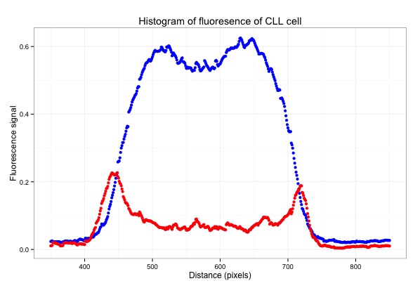
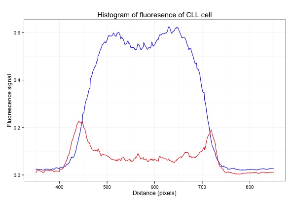
I've used EBImage to extract values and to generate this graph which shows the fluorescence of the pixels across the middle of the cell:

Here is the script with some plots that I generated along the way:

# EBImage - a Bioconductor package for analysing images

source("http://bioconductor.org/biocLite.R")

biocLite("EBImage")

library("EBImage")

library(ggplot2)

# the image is on Github
img <- readImage("https://raw.githubusercontent.com/brennanpincardiff/RforBiochemists/master/data/images/cllCell.jpg")
# the object created is a Large Image (24 Mb in this case!)

display(img)

# opens a window in a web browser and allows you to look at the image

print(img)

# shows some of the structure of the Large Image object.

dim(img)

# [1] 1024 1024    3   

# corresponds to x and y pixels of the image and then the number of colours for each pixel

# why do we want to do this?

# so that we can extract data out of the image and draw nice graphs. 

# to extract a value out of the Large Image use the imageData() function

# if you place the mouse over the image in the web browser, you see the name of the pixel. 

# we can extract the fluorescence value and plot the data

x <- imageData(img)[, 512, 3]

# this gives the values for colour 3 for the whole x line at the value of y = 512. 

# this is a list of 1024 numbers which can be plotted

plot(x)  

# the index at the bottom refers to the x values across the whole image. 

# using the web browser, I can choose the line across the middle of the cell

# extract a row of 100 pixels wide from left to right of the middle of the image.

# I chose to extract values from y pixel 425 to 545 which correspond to the middle of the cell

# colour 1

x10.col1 <- as.data.frame(imageData(img)[ ,425:525, 1])

plot(x10.col1$V5)  # plot one of the values

Plot one of the values (V5)

x10.col1$mean <- rowMeans(x10.col1[1:100])

plot(x10.col1$mean) # plot the mean

Plot the mean of 100 pixels

# colour 3

x10.col3 <- as.data.frame(imageData(img)[ ,425:525, 3])

x10.col3$mean <- rowMeans(x10.col3[1:100])

plot(x10.col3$mean, col = "blue")

lines(x10.col1$mean, col = "red")

Plot both colours using Base R

# assemble a data frame to allow us to use ggplot to plot the data..

m <- as.data.frame(x10.col1$mean)

m$col3 <- x10.col3$mean

# change the column names in the data frame

colnames(m) <- c("col1", "col3")

# make the basic ggplot object

p <- ggplot(data=m, aes(x=seq(1, length(col3)))) + 

     geom_line(aes(y = col3), colour = "blue") + 

     geom_line(aes(y = col1), colour = "red")

p  # show the plot

Plot both colours in ggplot2

# focus on just the cell

p <- ggplot(data=m, aes(x=seq(1, length(col3)))) + 

     geom_line(aes(y = col3), colour = "blue") + 

     geom_line(aes(y = col1), colour = "red") + 

     xlim(350,850) # focus on just the cell

p  # have a look

# gives Warning messages but these can be ignored.

Focus on the cell by limiting the x-axis.

# add some titles and a easy theme 

p <- p +  xlab("Distance (pixels)") +   #label x-axis

          ylab("Fluorescence signal") +    #label y-axis

          ggtitle("Histogram of fluoresence of CLL cell") +  #title

          theme_bw()     # a simple theme

p   # show the plot

Add titles and change the theme.

# plot points instead of lines...

q <- ggplot(data=m, aes(x=seq(1, length(col3)))) + 

  geom_point(aes(y = col3), colour = "blue") + 

  geom_point(aes(y = col1), colour = "red") + 

  xlim(350,850) +  

  xlab("Distance (pixels)") +   # label x-axis

  ylab("Fluorescence signal") +    # label y-axis

  ggtitle("Histogram of fluoresence of CLL cell") +  # add a title

  theme_bw()     # a simple theme

q   # show the plot

You have the plot at the top of the page....

Resources: 

• My first link to EBImage: http://www.r-bloggers.com/r-image-analysis-using-ebimage/
• Introduction to EBImage (PDF): http://bioconductor.org/packages/release/bioc/vignettes/EBImage/inst/doc/EBImage-introduction.pdf
• Reference manual for EBImage: http://bioconductor.org/packages/release/bioc/manuals/EBImage/man/EBImage.pdf
• http://www.cookbook-r.com/Graphs/Axes_(ggplot2)/
• http://stackoverflow.com/questions/13837565/how-to-plot-one-variable-in-ggplot