Using the Uniprot API to illustrate protein domains...

Update (2nd Nov 2017): I've updated the drawProteins package and it's  totally using ggplot so this script doesn't work. For more details see this blog post, please.

I'm a member of the Cardiff R User group and we're using R to explore APIs - application programming interfaces which allow R to access data. I chose the explore the API that allows me to download data from Uniprot, "a comprehensive, high-quality and freely accessible resource of protein sequence and functional information".

Tomorrow, we have our show and tell about what we have learned about using APIs with R. So in preparation and inspired by Stef Locke, the lead organiser for the Cardiff R User group, I have now created my first R package. The R package, called drawProteins, uses the API output to create a schematic protein domains.

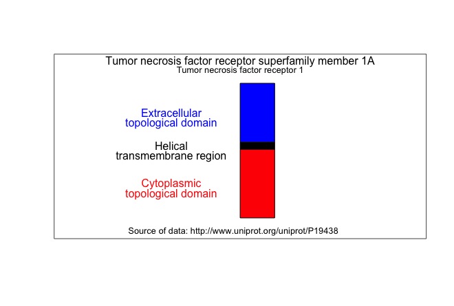
Here are two examples of the output. The first is a schematic of a single protein using Base R plotting (script below). The second example is a schematic of three proteins generated using ggplot2 (script in a little while).

Here is the script to plot a schematic of the transcription factor p65 (top panel):

SCRIPT START
# OK so I have to write some kind of a script to use the new 
# Uniprot API
# This is R-UserGroup homework for Thursday....

# references: https://www.ebi.ac.uk/proteins/api/doc/#!/proteins/search
# references: https://academic.oup.com/nar/article-lookup/doi/10.1093/nar/gkx237

# needs the package httr
# install.packages("httr")
library(httr)

# my package with functions for extracting and graphing
# might require: install.packages("devtools")
devtools::install_github("brennanpincardiff/drawProteins")
library(drawProteins)

# so I want to use the Protein API 
uniprot_acc <- c("Q04206")  # change this for your fav protein

# Get UniProt entry by accession 
acc_uniprot_url <- c("https://www.ebi.ac.uk/proteins/api/proteins?accession=")

comb_acc_api <- paste0(acc_uniprot_url, uniprot_acc)

# basic function is GET() which accesses the API
# requires internet access
protein <- GET(comb_acc_api,
           accept_json())

status_code(protein)  # returns a 200 means it worked

# use content() function from httr to give us a list 
protein_json <- content(protein) # gives a Large list
# with 14 primary parts and lots of bits inside

# function from my package to extract names of protein
names <- drawProteins::extract_names(protein_json)

# I like a visualistion so I want to draw the features of this molecule
# https://www.ebi.ac.uk/proteins/api/features?offset=0&size=100&accession=Q04206

# Get features 
feat_api_url <- c("https://www.ebi.ac.uk/proteins/api/features?offset=0&size=100&accession=")

comb_acc_api <- paste0(feat_api_url, uniprot_acc)

# basic function is GET() which accesses the API
prot_feat <- GET(comb_acc_api,
           accept_json())

status_code(prot_feat)  # returns a 200. 

# so to process this into a data.frame
prot_feat %>%
  content() %>%
  flatten() %>%
  drawProteins::extract_feat_acc() -> 
  features

# clean up for plotting
# focus on those that we want to plot...
features_plot <- features[features$length > 0, ]  
features_plot <- features_plot[complete.cases(features_plot),]
features_plot <- features_plot[features_plot$type!= "CONFLICT",]

# add colours 
library(randomcoloR)   # might need install
colours <- distinctColorPalette(nrow(features_plot)-1)
features_plot$col <- c("white", colours)

# now draw this...  with BaseR
# here is a function that does that....
drawProteins::draw_mol_horiz(names, features_plot)

# add phosphorylation sites
# get sites first. 
features %>%
  drawProteins::phospho_site_info() %>%
  drawProteins::draw_phosphosites(5, "yellow")  # 5 circle radius
text(250,0, "Yellow circles = phosphorylation sites", cex=0.8)

SCRIPT END

Resources

• Stef's 3 lines of code to make an R package: https://itsalocke.com/the-making-of-datasaurus/
• Another useful blog about writing a package: 
  http://tinyheero.github.io/jekyll/update/2015/07/26/making-your-first-R-package.html
• Key reference: Hadley Wickham's book on Packages
• Another R script exploring proteins: Drawing a simple phylogenetic tree of the human rel homology domain family

Drawing a cytokine receptor with R - TNFR1...

During my research, I have studied the pro-inflammatory cytokine TNF and its receptor, TNFR1. TNF and TNFR1 are involved in inflammatory diseases such as rheumatoid arthritis. As part of developing my skills drawing molecules with R, I have written this script to draw TNFR1.

I like to draw receptors vertically with the thought that the cell plasma membrane lies horizontal to the view. The height of the rectangles are proportional to the number of amino acids.

I took the data from the UniProt page for TNFR1. Here is the diagram.

The key functions involved are the 

• plot() function that creates the space to draw in
• rect() function that draws a rectangle
• text() function that adds text at a designated spot. 

Here is the script:

# START

# draw the Tumor Necrosis Factor Receptor 1 with R.

# draw it as a series of rectanges

# vertically rather than horizontal. 

# using the Uniprot webpage for the informaton

# http://www.uniprot.org/uniprot/P19438

# cut and paste from the XML page to create two objects

# first object is a list containing accession number and names

## Step 1: a list containing names 

# list of names...

names <- list(

  accession = c("P19438"),

  name = "TNR1A_HUMAN",

  protein.recommendedName.fullName = "Tumor necrosis factor receptor superfamily member 1A",

  protein.recommendedName.alternativeName = "Tumor necrosis factor receptor 1",

  protein.recommendedName.alternativeName.shortName = "TNF-RI",

  gene.name.primary = "TNFRSF1A",

  gene.name.synonym = "TNFAR",

  organism.name.scientific = "Homo sapiens"

)

## Step 2: getting the details of the molecule

# draw TNFR....

# Topological domain  22  211 Extracellular 189

# Transmembrane 212 234 Helical 22

# Topological domain 235 455 Cytoplasmic 220

# create the data frame with all the information. 

# cut and past from the XML page to make vectors

# features to plot 

types <- c("chain", "topological domain", "transmembrane region", "topological domain") 

description <- c("Tumor necrosis factor receptor superfamily member 1A, membrane form", "Extracellular", "Helical","Cytoplasmic")

begin <- c(22,22, 212, 235)

end <- c(455, 211, 234, 455)

subbegin <- 500 - begin # do these subtractions because we want to draw from top to bottom. 

subend <- 500 - end

col <- c("white", "blue", "black", "red")  # my decision - easy to change. 

# assemble vectors into a data frame

features <- data.frame(types, description, subbegin, subend, col)

# check the structure of the data frame

str(features)

# shows description and col to be factors - this will cause problems later...

# so change them now

features$description <- as.character(features$description)

features$col <- as.character(features$col)  

## step 3: draw the diagram - but vertically

screen.width <- 25 

screen.height <- 550  # this is a bit arbitrary

# we create a plot space to draw in....

plot(c(0, screen.width), 

     c(0, screen.height), 

     type= "n", 

     xlab = "", xaxt = 'n',   # suppress the x label and x axis

     ylab = "", yaxt = 'n')   # suppress the y label and y axis

# make the rectangles in a loop

for (i in 1:length(features$types) ) {

  rect(xleft   = screen.width/2,

       ytop    = features$subbegin[i],

       ybottom = features$subend[i],

       xright  = screen.width/2+2.5,

       col = features$col[i])

}

## Step 4: add text 

# text positioning all for horizontal code

# add text to the top of the illustration with the recommended name

text(screen.width/2, screen.height-2.5, names$protein.recommendedName.fullName, cex=1)

# and the alternative name

text(screen.width/2, screen.height-30, names$protein.recommendedName.alternativeName, cex=0.8)

# and source

text(12, 3, "Source of data: http://www.uniprot.org/uniprot/P19438", cex=0.8)

# add the descriptions of the features and source

# "chain" doesn't really help as a piece of text so going to leave this out. 

pos.text.y <- features$subbegin[2:4] + (features$subend[2:4] - features$subbegin[2:4])/2

pos.text.x <- 7.5

text(pos.text.x, pos.text.y, features$description[2:4], cex=1, col=features$col[2:4])

text(pos.text.x, pos.text.y - 35, features$types[2:4], cex=1, col=features$col[2:4])

## Step 5: add protein domains using shading as detailed on Uniprot

# add more TNF receptor domains:

begin <- c(43, 83, 126, 167, 356)

subbegin <- 500 - begin

end <- c(82, 125, 166, 196, 441)

subend <- 500 - end

description <- c("TNFR-Cys 1", "TNFR-Cys 2", "TNFR-Cys 3", "TNFR-Cys 4", "Death"  )

types <- c("repeat", "repeat", "repeat", "repeat", "domain")

density <- c(10, 10, 10, 10, 5)  # this gives lines in the shading

angle <- c(45, 135, 45, 135, 15) # this gives angles of the lines

features <- data.frame(types, description, subbegin, subend, density, angle)

features$description <- as.character(features$description)

# make the rectangles in a loop

for (i in 1:length(features$types) ) {

  rect(xleft   = screen.width/2,

       ytop    = features$subbegin[i],

       ybottom = features$subend[i],

       xright  = screen.width/2+2.5,

       lwd = 2,

       density = features$density[i],

       angle = features$angle[i]      

       )

}

# add the descriptions of the features

x <- length(features$types)

pos.text.y <- features$subbegin[1:x] + (features$subend[1:x] - features$subbegin[1:x])/2

pos.text.x <- 19.5

text(pos.text.x, pos.text.y, paste(features$description[1:x], features$types[1:x]), cex=1)

# SCRIPT END

Drawing a protein domain structure using R....

As a biochemist, I like a protein structure. Today, I have written a script to draw a protein structure for one of my favourite proteins, the NF-kappaB subunit, p65 - also known as Rel A. I've been measuring NF-kappaB since I published my first paper from my PhD in Trinity College Dublin (many years ago) and one of my most cited papers from Cardiff University is one of the first measurement of Rel A in a primary cells from a human cancer - chronic lymphocytic leukaemia.

The diagram is created using information from the Uniprot webpage for p65. It shows the domain structure for p65. Here is the diagram:

For those interested, RHD stands for Rel Homology Domain and TAD stands for Transactivation Domain. For more information, here's a link to the Wikipedia page.

Here is the script that draws the diagram:

SCRIPT START

# draw the NF-kappaB subunit, Rel A (p65) with R.

# draw it as a series of rectanges

# going from left to right. 

# using the Uniprot webpage for the informaton

# http://www.uniprot.org/uniprot/Q04206

# cut and paste from the XML page to create two objects

# first object is a list containing accession number and names

## Step 1: a list containing names and details 

# list of names...

names <- list(

  accession = c("Q04206"),

  name = "TF65_HUMAN",

  protein.recommendedName.fullName = "Transcription factor p65",

  protein.recommendedName.alternativeName = "Nuclear factor NF-kappa-B p65 subunit",

  protein.fullName = "Nuclear factor of kappa light polypeptide gene enhancer in B-cells 3",

  gene.name.primary = "RELA",

  gene.name.synonym = "NFKB3",

  organism.name.scientific = "Homo sapiens"

)

## step 2: create the data frame with all the information. 

# cut and past from the XML page to make vectors

# features to plot 

types <- c("chain", "domain", "region of interest", "short sequence motif", "short sequence motif") 

description <- c("Transcription factor p65", "RHD", "Activation domain","Nuclear localization signal", "9aaTAD")

begin <- c(1,19, 415, 301, 536)

end <- c(551, 306, 459, 304, 544)

col <- c("white", "blue", "red", "black", "orange")

# assemble vectors into a data frame

features <- data.frame(types, description, begin, end, col)

# check the structure of the data frame

str(features)

# shows description and col to be factors - this will cause problems later...

# so change them now

features$description <- as.character(features$description)

features$col <- as.character(features$col)  

# it will be better if we sort features in order of where they begin

features <- features[order(features$begin),]

## step 3: draw the diagram

screen.width <- max(features$end)

screen.height <- 25  # this is a bit arbitary

plot(c(-10, screen.width), 

     c(0, screen.height), 

     type= "n", 

     xlab = "Number of amino acids", 

     ylab = "", yaxt='n')    # suppress the y label and y axis

# make the rectangles in a loop

for (i in 1:length(features$types) ) {

  rect(xleft   = features$begin[i],

       ytop    = screen.height/2 + 2.5,

       ybottom = screen.height/2 - 2.5,

       xright  = features$end[i],

       col = features$col[i])

}

# add text to the top of the illustration with the recommended name

text(max(features$end)/2, screen.height-2.5, names$protein.recommendedName.fullName, cex=1.5)

# and the alternative name

text(max(features$end)/2, screen.height-5, names$protein.recommendedName.alternativeName, cex=1)

# add the descriptions of the features

pos.text.x <- features$begin[2:5] + (features$end[2:5] - features$begin[2:5])/2

pos.text.y <- c(screen.height/2 + 3.5, screen.height/2 - 3.5)

text(pos.text.x, pos.text.y, features$description[2:5], cex=1, col=features$col[2:5])

# add the accession number to the bottom smaller text and the source of the data

text(max(features$end)/2, 5 , paste("Uniprot Accession Number:", names$accession), cex=0.8)

text(max(features$end)/2, 3 , "Souce of data: http://www.uniprot.org/uniprot/Q04206", cex=0.8)