R for Biochemists: Africa

Two colleagues, Dr Mark Kelson and Dr David Gillipse, and I are going to Namibia as part of Project Phoenix. We are planning three days of R training. The materials are being developed and shared on Github as an open source teaching and learning resource.

Before I travel, I'm trying to learn a little more about where I'm going. As a first step, I've been drawing some maps of Namibia. Here are some of the maps:

Colourful map made by library(maps) - Map 1 below.

Map of regions of Namibia made by library(sp) - map 2 below

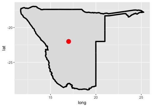
Map made with library(ggplot2) - map 3 below

I like using ggplot2 but, of course, there is a lot of personal preference. My next step is to add some data to a map...

## START SCRIPT

# exploring various ways to draw Namibia in R
# three ways....

## MAP 1 with library(maps)
library(maps) # Provides functions that let us plot the maps
library(mapdata) # Contains the hi-resolution points that mark out the countries.

# https://cran.r-project.org/web/packages/maps/maps.pdf
# gives a nice outline
map('worldHires',
c('Namibia'))

# add some context by adding more countries
map('worldHires',
c('Namibia', 'South Africa', 'Botswana', 'Angola',
'Zambia', 'Zimbabwe', 'Mozambique'))

# show all of Africa
# map the world but limit by longitude and latitude
map('worldHires',
xlim=c(-20,60), # longitude
ylim=c(-35,40)) # latitude

# focus on countries in Southern Africa
map('worldHires',
xlim=c(-10,50),
ylim=c(-35,10))

# add colour and a title
map('worldHires',
xlim=c(-10,50),
ylim=c(-35,10),
fill = TRUE,
col = c("red", "palegreen", "lightblue", "orange", "pink"))
title(main = "Simple map of Southern Africa")

## MAP 2 with library(sp) and downloaded GADM data
# this allows us to plot administrative regions inside Namibia
# https://www.students.ncl.ac.uk/keith.newman/r/maps-in-r-using-gadm
# http://biogeo.ucdavis.edu/data/gadm2.8/rds/NAM_adm1.rds

library(sp)

# download the file
link <- "http://biogeo.ucdavis.edu/data/gadm2.8/rds/NAM_adm1.rds"
download.file(url=link, destfile="file.rda", mode="wb")
gadmNab <- readRDS("file.rda") # special read file of format RDA

plot(gadmNab)

# plot with colour filled in, title and label.
plot(gadmNab, col = 'lightgrey', border = 'darkgrey')
title(main = "Map of admin regions inside Namibia")
points(17.0658, -22.5609,col=2,pch=18)
text(17, -22, "Windhoek")

## MAP 3 with library(ggplot2)
# the advantage is that we can add layers to our plot
# it gives us control
library(ggplot2)
# use map_data()function to create a data.frame containing the outline of Namibia
nab_map<-map_data("worldHires", region = "Namibia")

# create the object m with the map in it.
# colour Namibia (grey)
m <- ggplot() +
geom_polygon(data=nab_map, # geom_polygon draw shape fill
aes(x=long, # longitude
y=lat, # latitude
group=group),
fill="gray88")
m # show the object

# modify the object to add a thick black line
m <- m + geom_path(data=nab_map, # geom_path draw shape outline
aes(x=long, y=lat, group=group),
colour="black", # colour of line
lwd = 1.5) # thickness
m # show it again

# add the points on the plot telling us where the longitude and latitude of Windhoek
# note the data is coming from a different data.frame to the map
location <- data.frame(c(17), c(-22), c("Windhoek"))
colnames(location) <- c("longitude", "latitude", "location")

# add a point with the location
m <- m + geom_point(data=location,
aes(x=longitude, y=latitude),
colour="red", size = 5)
m # show the object

# add text at the same point
m <- m + geom_text(data = location,
aes(x=longitude,
y=latitude,
label = location)) # label has the text

# change the theme to make the map nicer
m <- m + theme_bw()

# add a title
m + ggtitle("Map of Namibia in ggplot")