Extracting an NFkappaB gene expression profile from published CLL gene expression data (Herishanu et al, Blood 2011)

Update: 18th October 2017 - Bioconductor is the place to get the Affymetrix annotation file.

This post is about exploring gene expression signatures. It was natural, for me, to start with the transcription factor, NFkappaB. On this blog, I have previously explored the principal component analysis of gene expression patterns from chronic lymphocytic leukaemia (CLL) cells published in Blood by Herishanu et al in 2011 - a key paper in this field.

In their paper, in Figure 5A, Herishanu et al focussed on a set of genes to investigate the gene signature for the transcription factor, NFkappaB. I found what they did very interesting and I wanted to reproduce their analysis using R and illustrate it here.

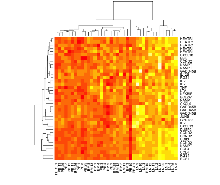
Here is my version of the heatmap, they showed in Figure 5A. My version has a little more information about the samples and the genes. The figures shows that the CLL cells from the lymph node (LN) have a higher NFkappaB gene signature is higher than the peripheral blood (PB) and the bone marrow (BM).

Heatmap showing the expression of selected NFkappaB regulated genes (listed on right) from CLL cells from peripheral blood (PB), bone marrow (BM) or lymph node (LN). Sample details on the bottom.

Here is the script I used to generate the data. To reproduce this, just cut and paste the script into R (or ideally R-Studio) and you should be able to generate the same figures.

START
# if required install packages
# install.packages("RCurl", "plyr", "heatmap3")

# the Affymetrix annotation file is located on Bioconductor
source("https://bioconductor.org/biocLite.R")
biocLite("hgu133plus2.db")   #installs the package
                   
# activate packages   
library(RCurl)     # to download data from internet
library(hgu133plus2.db)   # to link AffyIDs to gene names
library(plyr)   # to make a dataframe from a function
library(heatmap3) # one of many heatmap packages

# I want to extract the NF-kappaB gene profile and draw the first part of Figure 5. 
# I want to extract the values for a gene expression pattern
# need to extract it from the normalised data set.
# change colours to look more like the publication. 


# here is a link for all the normalised data from the paper (>50000 probes) 
x <- getURL("https://raw.githubusercontent.com/brennanpincardiff/RforBiochemists/master/data/herishanuMicroArrayDataNormalised.tsv")

# turn the data into a useful data.frame
data <- read.table(text = x, header = TRUE, sep = "\t")

# need to create a map that links AffyIDs to gene names
# http://bioconductor.org/packages/release/bioc/html/mygene.html
# U133 plus 2.0
# hgu133plus2.db

# https://www.bioconductor.org/help/workflows/annotation-data/
keytypes(hgu133plus2.db)

# SYMBOL is what we need

# map Affy IDs to Symbol
mapAffy_Symbol <- select(hgu133plus2.db, rownames(data), c("SYMBOL"))

# from Figure 5 there is a list of gene names
nfkb_genes <- c("RGS1", "CCND2", "NFKBIE", "CCL4", "CXCL13", "LTA", "CCL3", "BMEF1", "TNF", "CD83", "CXCL9", "BCL2A1", "DUSP2", "HEATR1", "CXCL10", "JUNB", "EBI2", "IL12B", "GADD45B", "EBI3", "ID2")

# test to see if we can find PROBEIDs which correspond to RGS1
mapAffy_Symbol[ which(mapAffy_Symbol$SYMBOL == "RGS1"),]
# works although there are more than one Affy ID per gene

# make a function to pull out probeID for a symbol
pullOutProbeID <- function(x){
  mapAffy_Symbol[ which(mapAffy_Symbol$SYMBOL == x),]
}

# use lapply to apply the function across the list of NFkB genes
lapply(nfkb_genes, pullOutProbeID)
# generates a list. 
# two of the list return nothing. 
# gene names have changed - I had to check the internet (GeneCards)
pullOutProbeID("NAMPT")  # BMEF1
pullOutProbeID("GPR183") # EBI2

# new list of NFkB genes with the two genes renamed. 
nfkb_genes2 <- c("RGS1", "CCND2", "NFKBIE", "CCL4", "CXCL13", "LTA", "CCL3", "NAMPT", "TNF", "CD83", "CXCL9", "BCL2A1", "DUSP2", "HEATR1", "CXCL10", "JUNB", "GPR183", "IL12B", "GADD45B", "EBI3", "ID2")


# this function from the package plyr
# ldply will return a data frame
genesAsAffyID <- ldply(nfkb_genes2, pullOutProbeID)


# make a function to pull out GeneExpvalues for AffyID
pullOutGeneExpVal <- function(x){
  subset(data, rownames(data) == x)
}

# test the function
pullOutGeneExpVal("202988_s_at")
# works

# extract the expression values
expVals <- ldply(genesAsAffyID$PROBEID, pullOutGeneExpVal)
View(expVals)
# good, I have extracted the values. 

# turn data.frame into a matrix so that we can draw a heatmap
expVals.m <- as.matrix(expVals)
# give it useful row names
rownames(expVals.m) <- genesAsAffyID$SYMBOL

# lets draw a heatmap using default settings from base R
heatmap(expVals.m)

# LN (lymph node) segregates well but
# PB (periperal blood) and BM (bone marrow) are mixed up

# we would like this order of the columns
sampl.order <- c("PB.1", "PB.2", "PB.3", "PB.4", "PB.4.1", "PB.8", "PB.9", 
  "PB.10", "PB.11", "PB.12", "PB.13", "PB.13.1",  "PB.25", "PB.26",
  "BM.1", "BM.2", "BM.3", "BM.4", "BM.8", "BM.9", 
  "BM.10", "BM.11", "BM.12", "BM.13",  "BM.25", "BM.26",
  "LN.1", "LN.2", "LN.3", "LN.4", "LN.8", "LN.9", 
  "LN.10", "LN.11", "LN.12", "LN.13",  "LN.25", "LN.26")

# reorder the matrix
expVals.m.o <- expVals.m[ , sampl.order]

heatmap(expVals.m.o,
        Colv = NA)     # don't reorder columns

# heatmap3 can look quite good. 
heatmap3(expVals.m.o,
         Colv = NA, # don't reorder columns
         Rowv = NA) # don't reorder rows either

# add some useful titles to the heatmap
title( main = "NFkappaB Gene Signature \n Figure 5A",
       sub  = "Source: Herishanu et al, \n Blood 2011 117:563-574; doi:10.1182/blood-2010-05-284984",
       cex.main = 1.5,
       cex.sub = 0.75, font.sub = 3, col.sub = "red")

# add text to top to label PB, BM and LN
# https://stat.ethz.ch/R-manual/R-devel/library/graphics/html/text.html
add.expr=text(x = 10, y = 118, "PB", cex = 1.5)
add.expr=text(x = 15, y = 118, "BM", cex = 1.5)
add.expr=text(x = 20, y = 118, "LN", cex = 1.5)

# add lines to the top - called segments
# https://stat.ethz.ch/R-manual/R-devel/library/graphics/html/segments.html
segments(6.8, 113, 12.3, 113, col = "green", lwd = 4)
segments(12.7, 113, 17.3, 113, col = "red", lwd = 4)
segments(17.7, 113, 22.2, 113, col = "blue", lwd = 4)

# this looks quite nice and seems similar to Figure 5A
# and a very good point to stop on for today. 

END


These resources were useful:

• http://www.genecards.org/cgi-bin/carddisp.pl?gene=GPR183&keywords=EBI2
• http://stackoverflow.com/questions/10590904/extracting-outputs-from-lapply-to-a-dataframe
• https://cran.r-project.org/web/packages/heatmap3/heatmap3.pdf
• http://stackoverflow.com/questions/19167586/add-text-on-heatmap-using-locator