Illustrating some R Fundamentals for VizBi 2016

I have surveyed the participants for my R tutorial at VizBi2016. The range of experience is a bit of a challenge. Some participants that have used R once or twice and others with plenty of experience. It's going to be a bit difficult to make the morning useful for everybody but I will try....

For the beginners, I'm going to start with this script which is designed to illustrate three of the fundamentals of R:

• functions
• objects
• packages

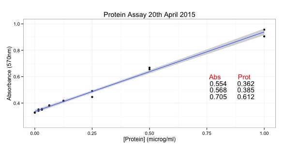
It's an expansion of the script to draw a graph of a protein assay with ggplot:

Here is the script:
# First script for VizBi2016
# written to illustrate the Fundamentals of R

## first 'Fundamental' is ** functions **
# functions do things!
# you know it's a function because it contains brackets

# c() is a function - sometimes called combine

## second 'Fundamental' is ** objects **
# objects contain data
# we make them with functions

# example:
# using the c() function to create the object prot
# Protein Concentrations
prot <- c(0.000, 0.016, 0.031, 0.063, 0.125, 0.250, 0.500, 1.000, 
          0.000, 0.016, 0.031, 0.063, 0.125, 0.250, 0.500, 1.000) 

# a function has arguments - always inside the brackets

# Absorbance from my protein assay
abs <- c(0.329, 0.352, 0.349, 0.379, 0.417, 0.491, 0.668, 0.956, 
         0.327, 0.341, 0.355, 0.383, 0.417, 0.446, 0.655, 0.905)

# these objects are called 'vectors' - key term

## now we are going ot play with some of these objects to 

#Calculate the line using the linear model function lm()
line <- lm(abs~prot)

# creates another kind of object - a list
# multiple parts with different type of data in each part

# too look at the object type line
line
summary(line)

# access particular parts of the object line
# using the $ dollar sign
# Equation of a line y = mx + c
# In our case abs = slope * prot + intercept
# ukn.prot = (abs - intercept)/slope
int <- summary(line)$coefficients[1]
slope <- summary(line)$coefficients[2]

# now calculate some unknown protein concs from absorbances
# put the unknowns into a vector
abs.ukns <- c(0.554, 0.568, 0.705)

# rearrange the equation of the line to ukn.prot = (abs - intercept)/slope
prot.ukns <- (abs.ukns - int)/slope

# CONCEPT ALERT - functions work on a vector of numbers


## graphing

# quick graph using base R
plot(prot, abs)
abline(line)

## BUT there is a better way!!

## third 'Fundamental' is ** packages **
# these are collections of functions that have been written by others
# these can be installed 
# install.packages("ggplot2")
# and then activated
library(ggplot2)

# Convert from one type of object to another
# another kind of object is a data.frame
# a bit like an Excel spreadsheet
# often when we import data we get a data frame
data <- as.data.frame(prot)
data$abs <- abs


# make a simple graph with ggplot
# step one - add the data and then the 'aesthetics' 
# key asthetics in this case x and y
p <- ggplot(data=data,          # specify the data frame with data
            aes(x=prot, y=abs)) # specify x and y for the graph

# creates a list and a blank plot

# add a type of graph 
p <- p + geom_point()

# show the graph
p

# add a line
p + stat_smooth(method = "lm")

# more detailed plot: 
p <- ggplot(data=data,          # specify the data frame with data
            aes(x=prot, y=abs)) +   # specify x and y for the graph
  geom_point() +          # make a scatter plot
  stat_smooth(method = "lm") +  # add a linear model line
  xlab("[Protein] (microg/ml)") +   # label x-axis
  ylab("Absorbance (570nm)") +    # label y-axis
  ggtitle("Protein Assay") +  # add a title
  theme_bw() +      # a simple theme
  expand_limits(y=c(0,1)) +    # customise the y-axis
  annotate(geom="text", x=0.85, y= 0.6, label="Abs         Prot",  color="red")

# put the answers on the graph
for (i in 1:length(abs.ukns)){
  p <- p + annotate(geom="text", x = 0.8, y = (0.6 - i/20), label=abs.ukns[i])
  p <- p + annotate(geom="text", x = 0.92, y = (0.6 - i/20), label=round(prot.ukns[i], 3))
}

p # show us the graph...

## To Learn from this script:
# run this script line by line yourself and see what happens.
# watch what happens

# make the plot object again and try some things...
p <- ggplot(data=data,          # specify the data frame with data
            aes(x=prot, y=abs)) # specify x and y for the graph

# try to change the colour of the points
p + geom_point(colour = "blue")

# try to change the size of the points
p + geom_point(size = 5, colour = "red")

# look at the documentation for geom_point
# http://docs.ggplot2.org/current/geom_point.html
# try some of the functions and see if you can make sense of them